Custom Search
|
|

|
||
 Then, taking the logarithm and squaring both sides of the equation:
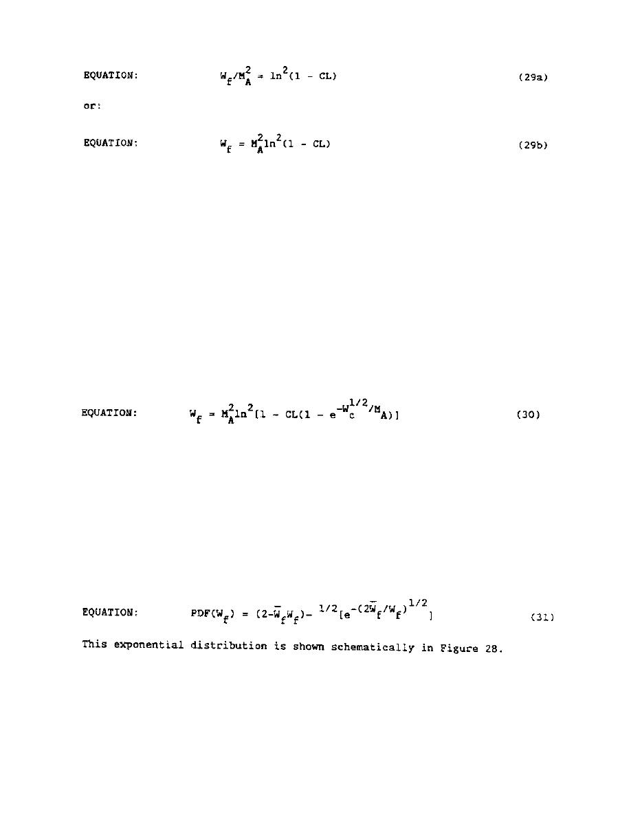
(a) Equation (29) can then be used to calculate the design
fragment weight for a prescribed probability or design confidence level.
(b) Note that, physically, the maximum possible value of Wf is
Wc, the total casing weight. For values of CL extremely close to 1, the
value of Wf calculated for Equation (29) may exceed Wc. In such cases,
Wf should be set equal to the casing weight. This inconsistency occurs
due to the use of an infinite distribution to describe a phenomenon which
obviously has a finite upper limit. The best example of this is obtained by
letting CL equal 1.0 in Equation (29). The infinite value obtained for Wf
illustrates that the chosen model is not physically reasonable for CL values
extremely close to 1.0. By imposing the condition that Wf be equal to
Wc for a probability of 1.0, an expression can be derived for a truncated
Wf distribution:
(c) Comparison of Equation (30) with Equation (29) for some
particular cases shows that the results are virtually identical, except for
CL values greater than 0.9999. Hence, the small benefit gained by the use
of Equation (30) does not justify its increased complexity and Equation (29)
is recommended for use in design.
(d) Finally, an expression can be derived for the probability
distribution function of fragment weights PDF(Wf), since:
(e) In order to implement these relationships for practical
design, a step-by-step procedure is outlined in this Section. Design charts
(Figures 29, 30, 31 and 32) and Table 4 are included to reduce the amount of
calculations.
2.08-52
|
 |
|
|
||